Welcome back
I didn't get much time working on the course in past 5 days!!!
Finally resuming today!
Today I reviewed Feature scaling part 1 and learned Feature scaling part 2 and Checking gradient descent for convergence.
The difficulty of the course is getter harder, 20mins video, I spent double time and needed to checking external articles to get better understanding.
Feature Scaling
Trying to understand what is "Feature Scaling"...
What are features and parameters in below formula?
hat of Price = w1x1 + w2x2 + b.
x1 and x2 are features, former one represents size of house, later one represents number of bedrooms.
w1 and w2 are parameters.
When a possible range of values of a feature is large, it's more likely that a good model will learn to choose a relatively small parameter value.
Likewise, when the possible values of the feature are small, like the number of bedrooms, then a reasonable value for its parameters will be relatively large like 50.
So how does this relate to grading descent?
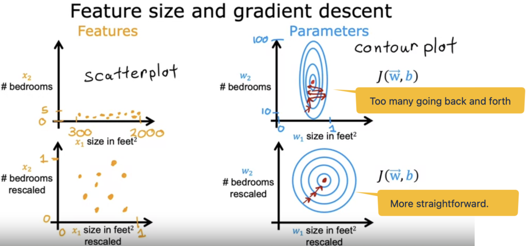
At the end of this video, Andrew explained that the features need to be re-scaled or transformed sl that the cost function J using the transfomed data would shape better and gradient descent can find a much more direct path to the global minimum.

When you have different features that take on very different ranges of values, it can cause gradient descent to run slowly but re scaling the different features so they all take on comparable range of values. because speed, upgrade and dissent significantly.
Andrew Ng
One key aspect of feature engineering is scaling, normalization, and standardization, which involves transforming the data to make it more suitable for modeling. These techniques can help to improve model performance, reduce the impact of outliers, and ensure that the data is on the same scale.
The Feature scaling part 2 mentioned why we need to scale. I did some google search and found out Feature Scaling: Engineering, Normalization, and Standardization (Updated 2024) is really good.
As a summary of the video, we know a few methods to do scaling:
- Divid with the maxium value of features.
- Mean Normalization
- Z-score normalization
As a rule of thumb, when performing feature scaling, you might want to aim for getting the features to range from maybe anywhere around negative one to somewhere around plus one for each feature x.
Andrew Ng
But these values, negative one and plus one can be a little bit loose.
If the features range from negative three to plus three or negative 0.3 to plus 0.3, all of these are completely okay.
If you have a feature x_1 that winds up being between zero and three, that's not a problem.
You can re-scale it if you want, but if you don't re-scale it, it should work okay too.
Too large or small, then should rescale.
Checking gradient descent for convergence
I learnt that using learning curve of J function to see whether the function is going convergence.
If graph of function J ever increases after one iteration, that means either Alpha is chosen poorly, and it usually means Alpha is too large, or there could be a bug in the code.
J of vector w and b should decrease as iteration increases.
If the curve has flattened out, this means that gradient descent has more or less converged because the curve is no longer decreasing.
Andrew said he usually found that choosing the right threshold epsilon was pretty difficult. He actually tended to look at learning curve, rather than rely on automatic convergence tests.
References
Terminology
| Term | Comments |
| Normalization | |
| Mean Normalization | |
| Z-score normalization | Involved to calculate "standard deviation σ". |
| standard deviation σ | It is a measure of how dispersed the data is in relation to the mean. Low, or small, standard deviation indicates data are clustered tightly around the mean, and high, or large, standard deviation indicates data are more spread out. Or if you've heard of the normal distribution or the bell-shaped curve, sometimes also called the Gaussian distribution, this is what the standard deviation for the normal distribution looks like. |
| Learning curve | It is difficult to tell in advance how many iterations gradient descent needs to converge, which is why you can create a learning curve. |
| Automatic Convergence Test | Another way to decide when your model is done training is with an automatic convergence test. If the cost J decreases by less than this number epsilon on one iteration, then you're likely on this flattened part of the curve that you see on the left and you can declare convergence. |