GeekCoding101

In logistic regression, the decision boundary is where z = w·x + b = 0. That is the point where the sigmoid outputs exactly 0.5, so the model switches between predicting 0 and 1. The cost function is built from logistic loss instead of squared error, because squared error combined with the sigmoid gives a bumpy, non-convex cost that gradient descent can get stuck in.
Those were my four topics for Day 10:
- Decision boundary
- Cost function for logistic regression
- Logistic loss
- Gradient descent implementation for logistic regression
Let’s continue!
GeekCoding101 · May 11, 2024 · Topics: machine-learning, notes, supervised-machine-learning
Decision boundary: where z = 0
Logistic regression passes a linear score through the sigmoid function:
z = w · x + bf(x) = g(z) = 1 / (1 + e^(-z))The output is between 0 and 1, and we read it as “probability that y = 1”. The usual rule is:
| Condition | Sigmoid output | Prediction |
|---|---|---|
| z > 0 | f(x) > 0.5 | 1 |
| z = 0 | f(x) = 0.5 | right on the boundary (neutral) |
| z < 0 | f(x) < 0.5 | 0 |
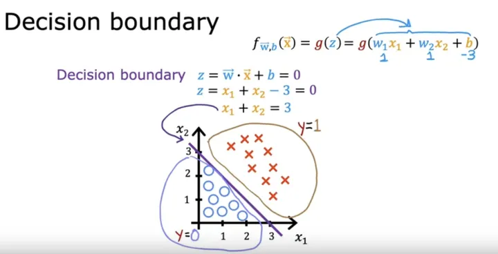
So the decision boundary is simply the set of points where z = 0. At that moment the sigmoid sits at its neutral position.
Andrew’s example with two features: take z = x1 + x2 - 3, so w1 = w2 = 1 and b = -3.
- Setting z = 0 gives the boundary line x1 + x2 = 3.
- Points above that line are predicted as 1.
- Points below it are predicted as 0.
The boundary doesn’t have to be a straight line. If you add polynomial features, the boundary becomes a curve. For example, z = x1² + x2² - 1 gives a circle of radius 1.
Cost function for logistic regression: the hard part
I want to say “Cost function for logistic regression” is the hardest part of week 3 I’ve seen so far. At first I didn’t get why the squared error cost function doesn’t work, or where the loss function came from. I had to re-watch the videos. The lab is also useful.
Here is what finally clicked for me.
Why squared error doesn’t work here
For linear regression, the squared error cost is a nice bowl shape (convex). Gradient descent rolls down to the single global minimum.
Plug the sigmoid into that same formula and the surface changes. The cost becomes non-convex, with lots of local minima. Gradient descent can settle into one of them and never reach the best parameters.
Logistic regression needs a cost function that suits its non-linear output. That starts with a different loss function.
Logistic loss
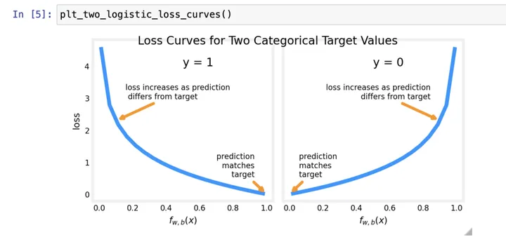
The loss for a single training example is:
if y = 1: L = -log(f(x))if y = 0: L = -log(1 - f(x))The intuition behind each case:
| True label | Prediction f(x) | Loss |
|---|---|---|
| y = 1 | close to 1 | close to 0 (good) |
| y = 1 | close to 0 | very large (heavily penalised) |
| y = 0 | close to 0 | close to 0 (good) |
| y = 0 | close to 1 | very large (heavily penalised) |
The more confident and wrong the model is, the bigger the penalty.
Simplified loss and the cost function
Because y is always 0 or 1, the two cases fold into one line:
L(f(x), y) = -y · log(f(x)) - (1 - y) · log(1 - f(x))- When y = 1, the second term disappears.
- When y = 0, the first term disappears.
The cost is the average loss over all m training examples:
J(w, b) = (1/m) · Σ L(f(x(i)), y(i))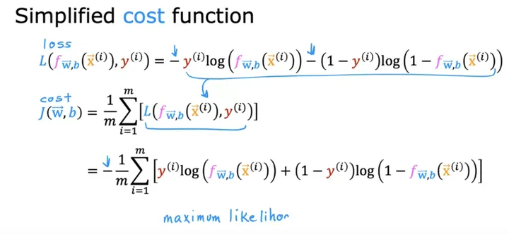
This cost function comes from statistics, from a principle called maximum likelihood estimation (MLE). It also has the property we lost with squared error: it is convex, so gradient descent can reach the global minimum.
Gradient descent implementation for logistic regression
The update rules look exactly like the ones for linear regression. Repeat until convergence, updating all parameters at the same time:
w_j = w_j - α · (1/m) · Σ (f(x(i)) - y(i)) · x_j(i)b = b - α · (1/m) · Σ (f(x(i)) - y(i))The difference is hidden inside f(x):
- In linear regression,
f(x) = w·x + b. - In logistic regression,
f(x) = sigmoid(w·x + b).
So it’s the same-looking algorithm applied to a different model. The tricks from linear regression still apply here too:
- feature scaling
- vectorization
- checking that the cost goes down each iteration
Here is a minimal NumPy version of the cost and gradient, roughly what the lab walks you through:
import numpy as np
def sigmoid(z):    return 1 / (1 + np.exp(-z))
def compute_cost(X, y, w, b):    f = sigmoid(X @ w + b)    return -np.mean(y * np.log(f) + (1 - y) * np.log(1 - f))
def compute_gradient(X, y, w, b):    m = X.shape[0]    err = sigmoid(X @ w + b) - y    dj_dw = X.T @ err / m    dj_db = np.mean(err)    return dj_dw, dj_db
Some thoughts of today
Honestly, it feels like it’s getting tougher and tougher.
I can still get through the equations and derivations alright. It’s just that as I age, I feel like my brain is not keeping up.
At the end of each video, Andrew always congratulates me with a big smile, saying I’ve mastered the content of the session. But deep down, I really think what he’s actually thinking is, “Ha, got you stumped again!”
To be fair, Andrew really does explain things superbly well. I hope someday I can truly master this knowledge and use it effortlessly.
Fighting!
FAQ
Why do we need a loss function in logistic regression? The loss measures how wrong the model is on one example. The cost function averages it over the dataset, which gives gradient descent something to minimise. Logistic regression needs a loss that fits its sigmoid output, which is why it uses logistic loss.
Why is the squared error cost function not used for logistic regression? With the sigmoid inside it, squared error produces a non-convex cost with many local minima. Gradient descent could get stuck. Logistic loss keeps the cost convex.
What is maximum likelihood? It is a statistical principle: choose the parameters that make the observed training labels most probable under the model. Applied to logistic regression, it produces the logistic loss cost function.
What’s the difference between “loss” and “cost”? “Loss” is measured on a single training example. “Cost” is the average of the loss across the entire dataset or a batch of training examples.
Is gradient descent for logistic regression the same as for linear regression? The update equations look identical. The difference is that f(x) is the sigmoid of w·x + b rather than w·x + b itself.
Keep reading
This post is part of my AI Machine Learning Journal series:
- Day 11, 12 – Overfitting! Unlocking the Last Key Concept in Supervised Machine Learning: overfitting vs underfitting, and fixing them with more data, simpler models or regularization.
- Day 9 – Master Gradient Descent and Binary Classification: back after being sick, revisiting gradient descent.
- Day 8 – Master Learning Rate and Feature Engineering: choosing the learning rate, the Jupyter lab, and feature engineering.
Thanks for reading! Feel free to check out my other posts or contact me via the links in the footer.