GeekCoding101

Overfitting is when a model learns the training data, including its noise, so closely that it predicts poorly on new data. You fix it in three ways: get more training data, use fewer features (a simpler model), or apply regularization, which shrinks the model’s parameters through a penalty term controlled by λ (lambda).
I finished the course! This was the last topic in Andrew Ng’s Supervised Machine Learning course, and I really enjoyed the learning experience. Here’s what I learned over days 11 and 12.
Overfitting vs underfitting at a glance
| Underfitting | Overfitting | |
|---|---|---|
| Also called | High bias (“preconception”) | High variance |
| On training data | Fits poorly | Fits very well, often almost perfectly |
| On new data | Predicts poorly | Predicts poorly |
| Typical cause | Model too simple for the pattern | Model too complex for the amount of data |
| Typical fix | More or better features, a more flexible model, smaller λ | More data, fewer features, regularization / larger λ |
Overfitting and underfitting are both signs that a model isn’t well tuned to the task. They come from opposite causes, so they need different fixes.
What is overfitting?
Overfitting happens when a model learns the details and noise in the training data to the point that it hurts performance on new data. The model is great at fitting the training set but can’t generalize from it to the broader population of data.
What you want is generalization: the learning algorithm should make good predictions even on brand-new examples it has never seen.
What is underfitting?
Underfitting is the opposite problem. The model is too simple to capture the pattern, so it does badly even on the training data.
Andrew describes this as the algorithm having a strong preconception (bias). For example, fitting a straight line to house prices that clearly curve as size grows is underfitting. The algorithm insists the data is linear, even though the data says otherwise.
You can’t fix underfitting with the tools for overfitting. More data won’t help a model that’s too simple for the pattern.
How to fix overfitting
The course gives three options:
- Get more training data. With more examples, the model can learn patterns that generalize instead of memorizing noise.
- Select features to include or exclude. Many features plus too little data is a recipe for overfitting, so using fewer features simplifies the model. The downside is that you might throw away features that were actually useful.
- Regularization. Keep all the features, but encourage the learning algorithm to shrink the parameter values. It doesn’t force any parameter to exactly 0. It just keeps every feature’s effect small.
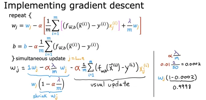
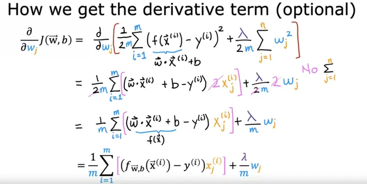
Below are two screenshots I captured from the course for my notes:
Regularization and λ (lambda)
Regularization adds a penalty term to the cost function. The penalty grows with the size of the parameters w, so the algorithm is pushed toward smaller values.
Regularized cost function, linear regression:
Regularized cost function, logistic regression:
Gradient descent updates. These have the same form for both models; only f differs:
What happens if λ is very large or very small?
- λ = 0 (or very small): there’s effectively no regularization, so the model can still overfit.
- λ very large: the algorithm shrinks every w close to 0, so f(x) ≈ b. That’s a flat line, and the model underfits.
- λ “just right”: the parameters stay small enough to avoid overfitting while the model still fits the data.
Does regularizing b make much difference?
In practice, not much. The penalty term only sums over w₁ … wₙ, and the convention in the course is to leave b out.
The formulas in Python
The hardest question on my list was to write down the formulas and explain how to implement them in Python. Here is a NumPy version of the regularized cost and gradient for linear regression:
import numpy as np
def compute_cost_linear_reg(X, y, w, b, lambda_=1.0):    """Regularized cost for linear regression. X: (m, n), y: (m,), w: (n,)"""    m = X.shape[0]    f_wb = X @ w + b                                 # predictions    cost = np.sum((f_wb - y) ** 2) / (2 * m)         # squared error part    reg = (lambda_ / (2 * m)) * np.sum(w ** 2)       # penalty on w only, not b    return cost + reg
def compute_gradient_linear_reg(X, y, w, b, lambda_=1.0):    m = X.shape[0]    err = (X @ w + b) - y    dj_dw = (X.T @ err) / m + (lambda_ / m) * w      # extra (λ/m)·w term    dj_db = np.sum(err) / m                          # b is not regularized    return dj_dw, dj_db
For logistic regression, the regularization part is the same. Replace the prediction with the sigmoid, f_wb = 1 / (1 + np.exp(-(X @ w + b))), and use the logistic loss in the cost. The gradient code stays the same.
Questions that helped me master the content
I use questions like these to check my understanding. Each one is answered in the sections above:
- What is overfitting (aka high variance)? How do you address it?
- What is underfitting?
- What is λ? How does a very large or very small value affect the learning algorithm?
- In practice, does regularizing b make much difference?
- Give an example of preconception (aka bias, or underfitting).
- What is generalization?
- (The hardest one) Write down all the formulas taught in the videos and explain how they could be implemented in Python.
FAQ
What’s the difference between overfitting and underfitting? Overfitting fits the training data too closely and fails on new data (high variance). Underfitting is too simple to fit even the training data (high bias).
How can I tell if my model is overfitting? It does very well on the training data but noticeably worse on examples it hasn’t seen.
What does the regularization parameter λ do? It controls how strongly large parameters are penalized. A larger λ means smaller parameters and a simpler model. Push it too far and the model underfits.
Should I regularize the bias term b? It usually makes little difference, and the course leaves b out of the penalty term.
Words from Andrew at the end
I want to say congratulations on how far you’ve come and I want to say great job for getting through all the way to the end of this video. I hope you also work through the practice labs and quizzes. Having said that, there are still many more exciting things to learn.
Awesome! I’m ready for the next machine learning journey. Thanks for reading! Feel free to check out my other posts, or reach out at /contact.