GeekCoding101

On Day 9 I finished the first coding assessment, which was implementing gradient descent for one-variable linear regression. Then I started week 3 of Andrew Ng’s Supervised Machine Learning course, where the topic switches to binary classification and logistic regression. Below are my notes on both: the gradient descent update rules, and the first ideas you need for classification (classes, the sigmoid, thresholds and decision boundaries).
May 9, 2024 · notes · supervised-machine-learning · machine-learning
A break due to sickness
Oh boy… I was sick for almost two weeks 🤒 After a short break, I’m back, and today I’m revisiting one of the core ideas in training models: gradient descent. Let’s dive back into the data-drenched depths where we left off, shall we? 🚀
The first coding assessment: gradient descent for one variable
Honestly, I couldn’t recall all of it at first. The assessment tests whether you can implement gradient descent for linear regression with a single feature. I walked back through the previous lessons and found this summary really helpful:
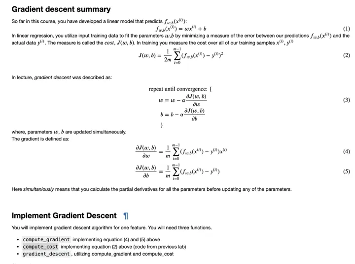
Here is the same idea written out, so it’s searchable and easy to copy.
The model and the cost function
| Piece | Formula | What it means |
|---|---|---|
| Model | fw,b(x) = w·x + b | A straight line with weight w and bias b |
| Cost | J(w,b) = (1 / 2m) · Σ (fw,b(x(i)) − y(i))² | Average squared error over m training examples |
| Goal | minimise J(w,b) | Find the w, b that fit the data best |
The update rules
Repeat until convergence:
- w := w − α · (1/m) · Σ (fw,b(x(i)) − y(i)) · x(i)
- b := b − α · (1/m) · Σ (fw,b(x(i)) − y(i))
Things to watch:
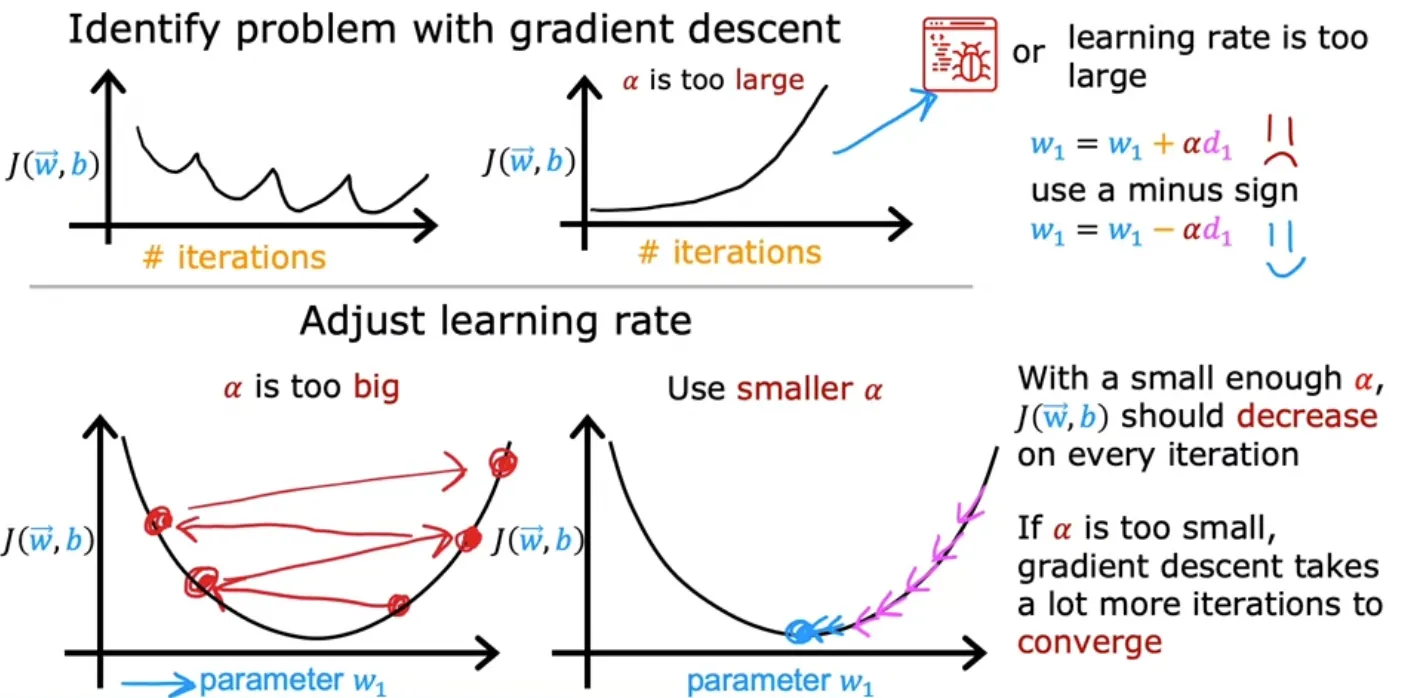
- α is the learning rate. If it’s too big, the cost can bounce around or blow up. If it’s too small, training crawls. (I covered choosing it on Day 8.)
- Update w and b simultaneously. Compute both gradients with the old values first, then assign both.
- Check the cost. If J(w,b) goes down every iteration, gradient descent is working.
A minimal sketch in Python
This is a plain illustration of the rules above, not the lab solution:
import numpy as np
def gradient_descent(x, y, w, b, alpha, num_iters):    m = len(x)    for _ in range(num_iters):        err = (w * x + b) - y          # prediction error for every example        dj_dw = (err * x).sum() / m    # gradient for w        dj_db = err.sum() / m          # gradient for b        w, b = w - alpha * dj_dw, b - alpha * dj_db   # simultaneous update    return w, b
The exercise really reinforced what I’d learned about gradient descent this week.
Getting into classification (week 3)
I started week 3, and it looks like it’ll be more interesting. Linear regression predicts a number. Classification predicts a category, and in binary classification there are only two categories.
Positive and negative classes
- y = 1 is the positive class. It means presence of the thing you’re looking for, not “good.”
- y = 0 is the negative class. It means absence, not “bad.”
In the course’s tumour example, a malignant tumour is the positive class and a benign one is the negative class. Detecting the cancer is “positive” even though it’s the bad outcome. (New English words for me: benign, malignant.)
Logistic regression and the sigmoid function
Logistic regression has “regression” in its name, but it’s a classification algorithm.
It takes the linear part you already know and squashes it into a range between 0 and 1 using the sigmoid function (also called the logistic function):
- z = w · x + b
- g(z) = 1 / (1 + e−z)
- fw,b(x) = g(w · x + b)
The output is read as a probability: the probability that y is 1, given input x and parameters w, b. In symbols, that’s P(y = 1 | x; w, b). If the model outputs 0.7, it’s saying there’s a 70% chance the example is in the positive class.
Threshold and decision boundary
To turn a probability into a yes/no answer, you pick a threshold, commonly 0.5:
| Model output | Prediction |
|---|---|
| fw,b(x) ≥ 0.5 | ŷ = 1 |
| fw,b(x) < 0.5 | ŷ = 0 |
Since g(z) ≥ 0.5 exactly when z ≥ 0, the line (or surface) where w · x + b = 0 is the decision boundary. Examples on one side are predicted positive, and examples on the other side are predicted negative.
I couldn’t focus for very long on this. I needed to pause after a few videos. More on decision boundaries and the logistic loss on Day 10.
Bye now 👋
FAQ
Why is logistic regression called “regression” if it’s used for classification? It is built on a linear regression–style expression (w · x + b). It then passes that through the sigmoid to produce a probability, which you threshold into a class. The name is historical; in practice it’s a classification method.
Does the “negative class” mean a bad result? No. Negative (y = 0) means the thing you’re detecting is absent, and positive (y = 1) means it’s present. A malignant tumour is the positive class.
What does the sigmoid function output? A value between 0 and 1. In logistic regression it’s interpreted as the probability that y = 1 for the given input.
Why do w and b have to be updated simultaneously in gradient descent? Both gradients should be computed from the same current parameters. If you update w first and then use the new w to compute b’s gradient, you’re no longer doing standard gradient descent.
This post is part of my Supervised Machine Learning Journey. Thanks for reading! Questions or corrections: contact page.